Restoration of a nonlinear function by a neural network with activation
Neural network with nonlinearity: theory
As we have shown in the previous tutorial, it is impossible to restore a nonlinear function with a neural network not containing nonlinearity. We will have to use the activation of neurons discussed in the Restoration of linear function by a single neuron to fix this:
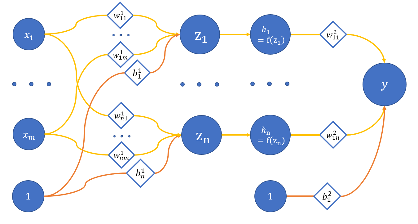
where
x_1 .. x_m - network input;
z_1 .. z_n - hidden layer neurons;
h_1 .. h_n - activation of the respective neurons of the hidden layer via the f function;
y - network output;
w_{ij}^{(l)} - weight of appropriate connections between neurons;
l - layer number, i - neuron on l + 1 layer, j - neuron on l layer;
b_i^{(l)} - bias on the respective layers.
We will take the network from the previous tutorial with three inputs and three neurons on the hidden layer. Then the only difference is activation after the hidden layer:
where h_j = f(z_j).
The gradient calculation for the parameter will change accordingly
We take ReLU as an activation function, where:
Neural network with nonlinearity: code
Start of the script:
import numpy as np
import matplotlib.pyplot as plt


def show(x, y, pred=None, title=None):
        plt.plot(x, y, linewidth=5, color="black", antialiased=True, label="True values")

        if pred is not None:
                plt.plot(x, pred, linewidth=2, color="orange", antialiased=True, label="Predicted values")
        if title is not None:
                plt.title(f'{title}')
        plt.legend()
        plt.show()


def showSubplots(x, y, *args, title=None):
        fig = plt.figure(1, figsize=[10.4, 4.8])

        for i, arg in enumerate(args):
                i += 1
                ax = fig.add_subplot(int("12{}".format(i)))

                ax.plot(x, y, linewidth=5, color="black", antialiased=True, label="True values")

                yp = arg["y"]
                name = arg["name"]
                color = arg["color"]

                ax.plot(x, yp, linewidth=2, color=color, antialiased=True, label="{}".format(name))

                ax.legend()
        if title is not None:
                fig.suptitle(f'{title}')
        fig.show()
Take classes Linear and Net from tutorial Restoring a linear function by a neural network:
class Linear:
    def __init__(self, insize, outsize, name=None):
        self.w = np.random.randn(insize, outsize)
        self.b = np.zeros((outsize, ))

        self.inData = None
        self.data = None

        self.grad = None

        self.name = name


    def __call__(self, data):
        return self.forward(data)


    def forward(self, data):
        self.inData = data
        self.data = np.dot(data, self.w) + self.b

        return self.data


    def backward(self, grad):
        delta = np.dot(grad, self.w.T)
        self.grad = grad

        return delta

    def update(self, lr=0.1):
        self.w -= np.dot(self.inData.T, self.grad) * lr
        self.b -= np.dot(self.grad.T, np.ones(self.grad.shape[0], )) * lr
class Error:
    @staticmethod
    def value(true, pred):
        return 0.5 * np.mean((true - pred) ** 2)


    @staticmethod
    def grad(true, pred):
        c = 1 / np.prod(true.shape)
        return -(true - pred) * c

class Net:
    def __init__(self):
        self.layers = []


    def __call__(self, data):
        return self.predict(data)


    def __getitem__(self, item):
        return self.layers[item]


    def append(self, layer):
        self.layers.append(layer)
    def backward(self, grad):
        for layer in self.layers[::-1]:
            grad = layer.backward(grad)


    def update(self, lr):
        for layer in self.layers:
            layer.update(lr)


    def predict(self, data):
        for layer in self.layers:
            data = layer.forward(data)

        return data


    def optimize(self, data, target, lr):
        prediction = self(data)

        #print("Simple net error {}".format(Error.value(target, prediction)))

        grad = Error.grad(target, prediction)

        self.backward(grad)
        self.update(lr)
X = np.linspace(-3, 3, 1024, dtype=np.float32).reshape(-1, 1)

def func(x):
        from math import sin
        return 2 * sin(x) + 5

f = np.vectorize(func)
Y = f(X)
A new class - Activation is added. It implements ReLU activation:
class Activation:
    def __init__(self, name="relu"):
        self.name = name

        self.inData = None
        self.data = None

        self.grad = None


    def forward(self, data):
        self.inData = data

        self.data = data * (data > 0)

        return self.data


    def backward(self, grad):
        self.grad = (self.data > 0) * grad

        return self.grad


    def update(self, lr):
        pass
Network training
We introduce a new trick for a nonlinear function - data mixing. We used to form a batch from values that follow each other in a sequence, but now a batch can contain points from different ends of the function definition area:
def trainNet(size, steps=1000, batchsize=10, learnRate=1e-2):
    np.random.seed(1234)

    net = Net()
    net.append(Linear(insize=1, outsize=size, name="layer_1"))
    net.append(Activation(name="act_layer"))
    net.append(Linear(insize=size, outsize=1, name="layer_2"))

    predictedBT = net(X)

    XC = X.copy()
    perm = np.random.permutation(XC.shape[0])
    XC = XC[perm, :]

    for i in range(steps):
        idx = np.random.randint(0, 1000 - batchsize)
        x = XC[idx:idx + batchsize]
        y = f(x).astype(np.float32)

        net.optimize(x, y, learnRate)

    predictedAT = net(X)

    showSubplots(
        X,
        Y,
        {
            "y": predictedBT,
            "name": "Net results before training",
            "color": "orange"
        },
        {
            "y": predictedAT,
            "name": "Net results after training",
            "color": "orange"
        }
    )
trainNet(5, steps=1000, batchsize=100)
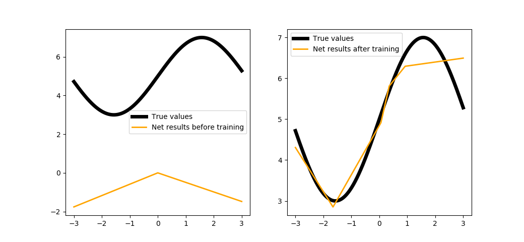
As you can see, the network intends to describe our function, and each neuron in the hidden layer is responsible for its own section of the curve. It would be a logical step to try increasing the number of neurons:
trainNet(100, steps=1000, batchsize=100)
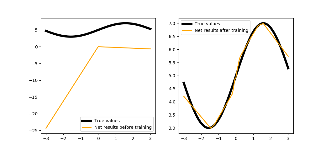
Looks better, but still not accurate. We could increase the number of steps to improve the quality, but that would take a too long, so it is time to use some more powerful tools of the PuzzleLib library.
Implementing the library tools
Please mind that this time we train the network not by steps (running a single batch), but by epochs (running the entire dataset), and we also pick a more advanced optimizer:
def trainNetPL(size, epochs, batchsize=10, learnRate=1e-2):
    from PuzzleLib.Modules import Linear, Activation
    from PuzzleLib.Modules.Activation import relu
    from PuzzleLib.Containers import Sequential
    from PuzzleLib.Optimizers import MomentumSGD
    from PuzzleLib.Cost import MSE
    from PuzzleLib.Handlers import Trainer
    from PuzzleLib.Backend.gpuarray import to_gpu

    np.random.seed(1234)

    net = Sequential()
    net.append(Linear(insize=1, outsize=size, initscheme="gaussian"))
    net.append(Activation(activation=relu))
    net.append(Linear(insize=size, outsize=1, initscheme="gaussian"))

    predictedBT = net(to_gpu(X)).get()

    cost = MSE()
    optimizer = MomentumSGD(learnRate)
    optimizer.setupOn(net)

    trainer = Trainer(net, cost, optimizer, batchsize=batchsize)

    show(X, Y, net(to_gpu(X)).get())

    XC, YC = X.copy(), Y.copy()
    perm = np.random.permutation(XC.shape[0])
    XC = XC[perm, :]
    YC = YC[perm, :]

    for i in range(epochs):
        trainer.trainFromHost(XC.astype(np.float32), YC.astype(np.float32), macroBatchSize=1000,
                                onMacroBatchFinish=lambda train: print("PL module error: %s" % train.cost.getMeanError()))

    net.evalMode()

    predictedAT = net(to_gpu(X)).get()

    showSubplots(
        X,
        Y,
        {
            "y": predictedBT,
            "name": "PL net results before training",
            "color": "orange"
        },
        {
            "y": predictedAT,
            "name": "PL net results after training",
            "color": "orange"
        }
    )
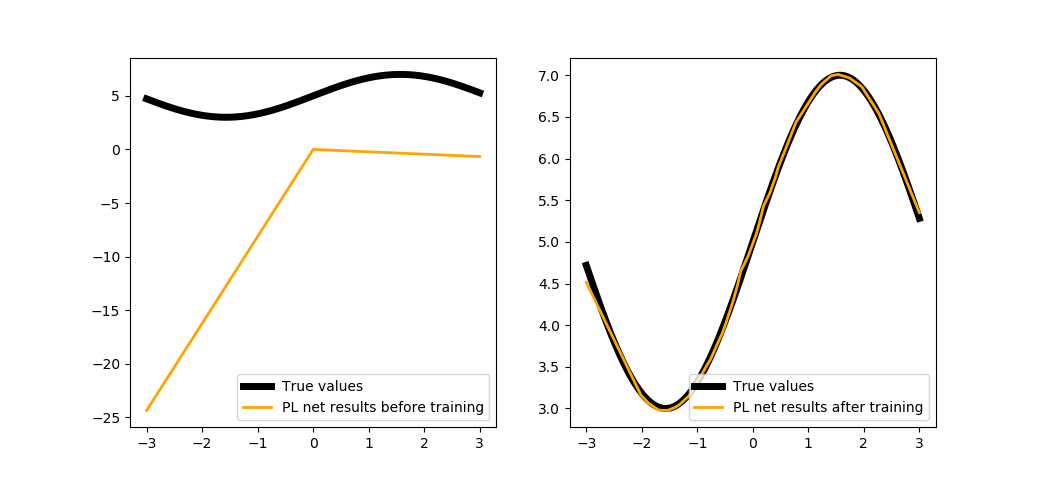
Conclusion
We can conclude that any framework for deep learning is generally a library for automatic differentiation of computational graphs, no magic involved here. We hope that by filling the gaps in understanding the work of neural networks we managed to help the reader get more confident, so you could perhaps even participate in the development of the PuzzleLib library by writing your own modules.