Training CIFAR classifier
Introduction
In this tutorial, we will learn how to train a color image classifier for 10 classes.
We strongly advise that you complete Training the MNIST classifier first.
Training sample
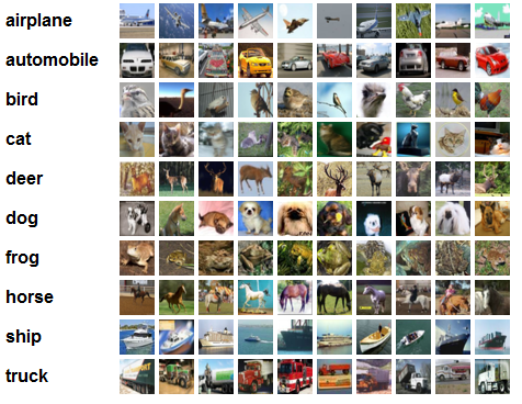
Download the CIFAR dataset from the original University of Toronto website , where this dataset was collected. This dataset contains 60,000 color images of size 32x32. Each image shows an object falling into one of the ten types: airplane, automobile, bird, cat, deer, dog, frog, horse, ship, truck. There are exactly 6000 images per class.
This dataset, like MNIST, is considered to be a basic one in machine learning: it tests various machine learning methods before they could be scaled.
Implementation in library tools
In this tutorial the script starts almost the same way as in the MNIST tutorial:
import os
import math

import numpy as np

from PuzzleLib.Datasets import Cifar10Loader

from PuzzleLib.Containers import Sequential
from PuzzleLib.Modules import Conv2D, MaxPool2D, Activation, Flatten, Linear
from PuzzleLib.Modules.Activation import relu
from PuzzleLib.Handlers import Trainer, Validator
from PuzzleLib.Optimizers import MomentumSGD
from PuzzleLib.Cost import CrossEntropy

from PuzzleLib.Visual import showImageBasedFilters, showFilters
There are new imports of the math library and the showImageBasedFilters function, we will explain their presence later. Also, the CIFAR loader Cifar10Loader, similar in meaning to the MNIST loader, is present in the imports.
Download data:
cifar10 = Cifar10Loader()
path = "../TestData/"
data, labels = cifar10.load(path=path)
data, labels = data[:], labels[:]
print("Loaded cifar10")

np.random.seed(1234)
Important
Please do not forget to replace the path variable with the path where you have unpacked the archives with the dataset.
Building the network
The Sequential container interconnects the modules:
seq = Sequential()
And now you will see the first differences from the MNIST tutorial, which you should pay close attention to. The network architecture will be quite the same, but mind the parameters set for the modules:
seq.append(Conv2D(3, 32, 5, pad=2, wscale=0.0001, initscheme="gaussian"))
The pad (padding) parameter tells the convolutional layer what margin to make on the sides of the photo. In our case that means that the photo is enlarged by 2 pixels on the left, right, top, and bottom, and the new pixels are filled with zeros (this is true for each of the input data maps, i.e. in the case of RGB, each of the R, G, and B maps will be enlarged).
This is necessary, for instance, for better processing of the map edges: after all, the convolutional layer filter without padding will rest on the edge of the photo. With padding the filter window is allowed to breach the map a little, capturing the zeros added there.
The wscale and initscheme parameters are responsible for what values the weights of the created layer will have at the very beginning, before the training process. The "gaussian" value will tell the layer to take the weights as random normal, with a default mean of 0.0, and the variance equal to wscale.
Why have we selected such parameters here? Similar architecture was invented by Krizhevsky (this very option goes under the slogan "26% in 80 seconds on the Fermi-generation Nvidia GPU").
Adding a maxpool to parameters other than the default parameters:
seq.append(MaxPool2D(size=3, stride=2))
The first parameter is the filter size, and the second parameter is the filter step for the photo. By default, they are 2 and 2, respectively.
This part goes without any innovations:
seq.append(Activation(relu))

seq.append(Conv2D(32, 32, 5, pad=2, wscale=0.01, initscheme="gaussian"))
seq.append(MaxPool2D(size=3, stride=2))
seq.append(Activation(relu))

seq.append(Conv2D(32, 64, 5, pad=2, wscale=0.01, initscheme="gaussian"))
seq.append(MaxPool2D(size=3, stride=2))
seq.append(Activation(relu))

seq.append(Flatten())
Yet the initialization of the linear layer differs significantly from the MNIST tutorial:
seq.append(Linear(seq.dataShapeFrom((1, 3, 32, 32))[1], 64, wscale=0.1, initscheme="gaussian"))
Here the data returned by the dataShapeFrom method defines the size of the linear layer. Many neural layer modules have this method: it receives input size (number of images, number of maps in the image, map height, map width), and outputs the data size after passing it through the layer. For example, the Activation layer will return the same size that it received when accessing this method, since the activation layers do not change the size of the data, but the convolutional layer or the maxpool layer can change it.
To avoid all the bother with the size of the data before entering the new layer, we asked seq for the size of the data at the output, and then took the component of size 1 (the size is 4 numbers, for example, (1, 3, 32, 32)): the complete dimensionality of each data item (i.e., component 0 is the number of training samples, component 1 - sample size, component 2 - number 1, component 3 - number 1, as Flatten has flattened everything) lies in this component after the Flatten method
We want a vector of size 64 at the output of the linear layer and specify the initialization of weights explicitly.
And finally, the last blocks of the network:
seq.append(Activation(relu))

seq.append(Linear(64, 10, wscale=0.1, initscheme="gaussian"))
Training preparations and network training
Selecting the loss function, the optimizer, and installing it on the network:
optimizer = MomentumSGD()
optimizer.setupOn(seq, useGlobalState=True)
optimizer.learnRate = 0.01
optimizer.momRate = 0.9

cost = CrossEntropy(maxlabels=10)

trainer = Trainer(seq, cost, optimizer)

validator = Validator(seq, cost)
Same as in the MNIST tutorial, but for one new line:
currerror = math.inf
Which creates a currerror variable, that will store the network error on the data in each epoch. We can use it to change the learning rate learnRate for our optimizer. First, we set the error equal to positive infinity, because we want to compare the error with something already in the zero epoch of training.
Network training
Starting training on 25 epochs:
for i in range(25):
    trainer.trainFromHost(data[:50000], labels[:50000], macroBatchSize=50000,
                            onMacroBatchFinish=lambda train: print("Train error: %s" % train.cost.getMeanError()))
    valerror = validator.validateFromHost(data[50000:], labels[50000:], macroBatchSize=10000)
    print("Accuracy: %s" % (1.0 - valerror))
Then come the lines that we have not met before:
    if valerror >= currerror:
        optimizer.learnRate *= 0.5
        print("Lowered learn rate: %s" % optimizer.learnRate)

    currerror = valerror
This is a rule of thumb, that indicates when to lower the training rate.
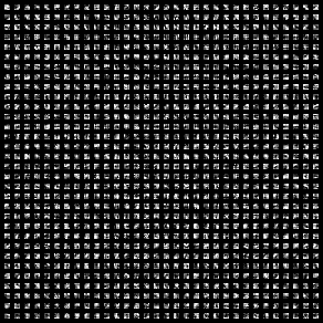
After that, since CIFAR is colored, we can display the first network layer in color. Which means that for each of the three RGB channels, we take the corresponding filters, and then apply them to each other (filters R - as red, G - as green and B - blue). This can only be done for the first layer, since further the binding to one of the RGB colors is lost. The showImageBasedFilters method performs this procedure for displaying filters for the first layer:
showImageBasedFilters(seq[0].W.get(), os.path.join(path, "conv1.png"))
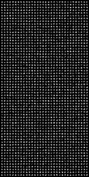
In addition to the first layer, we output the second and third convolutional layers to the file:
    showFilters(seq[3].W.get(), os.path.join(path, "conv2.png"))
    showFilters(seq[6].W.get(), os.path.join(path, "conv3.png"))
After 25 epochs of training, the following images are obtained:

The accuracy with which the network has learned to classify images:
print("Accuracy:", Accuracy)
Accuracy: 0.7629
As you can see, this is a much more difficult task for neural networks than MNIST. The network was able to identify correctly only 76% of the images.