Activation
Description
General information
This module implements the layer activation operation.
The activation function is a given mathematical operation on data that adds non-linearity to the transformation of a neural network.
Implemented Activation Functions
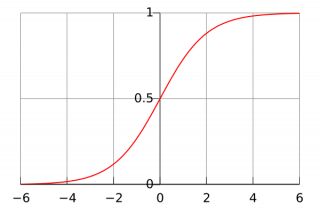
Sigmoid
It takes an arbitrary real number at the input, and at the output it returns a real number in the range from 0 to 1.
It is calculated by the formula:
Graph of the function:
Pros:
- infinitely differentiable smooth function
Cons:
-
saturation of the sigmoid leads to damping of the gradient: in the process of back propagation of the error, the local gradient, which can be very small, is multiplied by the general one, and in this case it zeroes it. Because of this, the signal hardly passes through the neuron to its weights and, recursively, to its data;
-
the sigmoid output is not centered around zero: in subsequent layers, the neurons will receive values that are also not centered around zero, which affects the dynamics of gradient descent.
Tanh
It takes an arbitrary real number at the input, and at the output it returns a real number in the range from –1 to 1.
It is calculated by the formula:
Graph of the function:
Pros:
- infinitely differentiable smooth function
- centered around zero
Cons:
- saturation problem
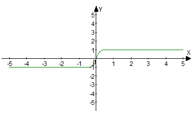
ReLU
Implements a threshold transition at zero. It is defined on the interval [0, + ∞). At the moment, relu is one of the most popular activation functions that has many modifications.
It is calculated by the formula:
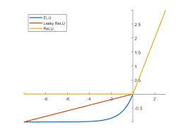
Graphs of this function and its two modifications:
Pros:
- computational simplicity
- fast stochastic gradient convergence
Cons:
- fading gradient (eliminated by choosing the appropriate learning speed)
- not a smooth function
LeakyReLU
Modification of relu with the addition of a small constant α. When the argument is negative, the value of the function is quite close to zero, but not equal to it. It is defined on the interval (-∞, + ∞).
It is calculated by the formula:
The graph is shown in the image above.
Pros:
- computational simplicity
- fast stochastic gradient convergence
Cons:
- fading gradient
- not a smooth function
ELU
Smooth modification of relu and leakyRelu. It is defined on the interval [-α, + ∞).
It is calculated by the formula:
The chart was given above.
Pros:
- computational simplicity
- fast stochastic gradient convergence
- smooth function
Cons:
- fading gradient
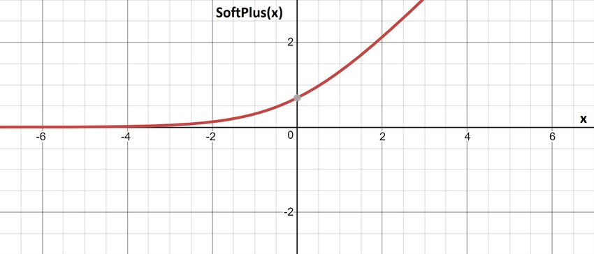
SoftPlus
Smooth activation function. It is defined on the interval [0, + ∞).
It is calculated by the formula:
It is calculated by the formula:
Pros:
- smooth infinitely differentiable function
Cons:
- not centered around zero
- fading gradient
Additional sources
- Wikipedia article with a large comparative characteristic table of all popular activation functions.
Initializing
def __init__(self, activation, slc=None, inplace=False, name=None, args=()):
Parameters
| Parameter | Allowed types | Description | Default |
|---|---|---|---|
| activation | str | Type of activation | - |
| slc | slice | The slice according to which the activation function will be calculated | None |
| inplace | bool | If True, the output tensor will be written in memory in the place of the input tensor | False |
| name | str | Layer name | None |
Explanations
activation - defines the selected activation function. Currently implemented activation functions are: "sigmoid", "tanh", "relu", "leakyRelu", "elu", "softPlus", "clip".
inplace - a flag showing whether additional memory resources should be allocated for the result. If True, then the output tensor will be written in the place of the input tensor in memory, which can negatively affect the network, if the input tensor takes part in calculations on other branches of the graph.
Examples
Necessary imports.
import numpy as np
from PuzzleLib.Backend import gpuarray
from PuzzleLib.Modules import Activation
Info
gpuarray is required to properly place the tensor in the GPU.
Let us form the visual data.
np.random.seed(123)
h, w = 3, 3
data = gpuarray.to_gpu(np.random.randint(-10, 10, (h, w)).astype(np.float32))
print(data)
[[  3.  -8.   -8.]
 [ -4.   7.    9.]
 [  0.  -9.  -10.]]
Suppose we are interested in a sigmoid as an activation function. Let us initialize the object and send data to it.
act = Activation('sigmoid')
print(act(data))
[[0.95257413  0.00033535017  0.00033535017]
 [0.01798621  0.999089       0.99987662  ]
 [0.5         0.00012339462  0.000045397865 ]]
ReLU:
act = Activation("relu")
print(act(data))
[[3. 0. 0.]
 [0. 7. 9.]
 [0. 0. 0.]]