Restoring a linear function by a neural network¶

Neural network: theory¶

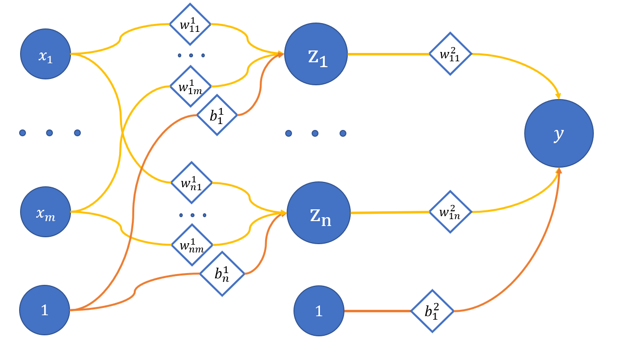
In the previous tutorial we discussed a simplified neuron (with one input and no activation) convenient for restoring a linear function. In this tutorial, we will complicate the architecture of our model and create a network of neurons with one hidden layer (the number of outputs will still equal one):

Figure 1. Network diagram with one hidden layer

where

$x_1 .. x_m$ - network input;

$z_1 .. z_n$ - neurons of the hidden layer;

$y$ - network output;

$w_{ij}^{(l)}$ - weights of the corresponding connections between neurons;

$l$ - layer number, $i$ - neuron on $l + 1$ layer, $j$ - neuron on the $l$ layer;

$b_i^{(l)}$ - biases on the corresponding layers.

Now we will look at a network with three inputs and three hidden neurons, e.g. $n = m = 3$ . Сalculating the values of hidden neurons:

$z_i = \sum_{j=1}^{m} w_{ij}^{(1)}x_j + b_i^{(1)}$

$z = W^{(1)}x + b^{(1)} = \begin{pmatrix} w_{11}^{(1)} & w_{12}^{(1)} & w_{13}^{(1)} \\ w_{21}^{(1)} & w_{22}^{(1)} & w_{23}^{(1)} \\ w_{31}^{(1)} & w_{32}^{(1)} & w_{33}^{(1)} \end{pmatrix} \begin{pmatrix} x_1 \\ x_2 \\ x_3 \end{pmatrix} + \begin{pmatrix} b_{1}^{(1)} \\ b_{2}^{(1)} \\ b_{3}^{(1)} \end{pmatrix} = \begin{pmatrix} w_{11}^{(1)}x_1 + w_{12}^{(1)}x_2 + w_{13}^{(1)}x_3 + b_{1}^{(1)} \\ w_{21}^{(1)}x_1 + w_{22}^{(1)}x_2 + w_{23}^{(1)}x_3 + b_{2}^{(1)} \\ w_{31}^{(1)}x_1 + w_{32}^{(1)}x_2 + w_{33}^{(1)}x_3 + b_{3}^{(1)} \end{pmatrix} = \begin{pmatrix} z_{1} \\ z_{2} \\ z_{3} \end{pmatrix}$

Calculating the output neuron value:

$y = \sum_{j=1}^{n} w_{1j}^{(2)}z_j + b_1^{(2)} = W^{(2)}z + b^{(2)} = w_{11}^{(2)}z_1 + w_{12}^{(2)}z_2 + w_{13}^{(2)}z_3 + b_{1}^{(2)}$

How do we solve the optimization problem for such model? Take the same loss function:

$J(\theta) = \frac{1}{2N}\sum_{i=1}^N(y_i-y_i^p)^2$

Now we need to understand how to calculate the gradient from it. There should be no problems with the parameters of the output layer. The formulas here are similar to those we had for a simple neuron:

$\begin{equation} \frac{\partial{J}}{\partial{w_{1j}^{(2)}}} = \frac{\partial{J}}{\partial{y}}\frac{\partial{y}}{\partial{w_{1j}^{(2)}}} \end{equation}$

As already shown in the previous tutorial:

$\begin{equation} \frac{\partial{J}}{\partial{y}} = -(y-y^p) \end{equation}$

$\begin{equation} \frac{\partial{y}}{\partial{w_{1j}^{(2)}}} = z_j \end{equation}$

We must understand that $z_j$ is a known value, since we get it at the forward propagation.

What about the hidden layer parameters? We need to learn more about the value of the $y$ output layer:

$y = w_{11}^{(2)}z_1 + w_{12}^{(2)}z_2 + w_{13}^{(2)}z_3 + b_{1}^{(2)} = w_{11}^{(2)} \cdot (w_{11}^{(1)}x_1 + w_{12}^{(1)}x_2 + w_{13}^{(1)}x_3 + b_{1}^{(1)}) + w_{12}^{(2)} \cdot (w_{21}^{(1)}x_1 + w_{22}^{(1)}x_2 + w_{23}^{(1)}x_3 + b_{2}^{(1)}) + w_{13}^{(2)} \cdot (w_{31}^{(1)}x_1 + w_{32}^{(1)}x_2 + w_{33}^{(1)}x_3 + b_{3}^{(1)}) + b_{1}^{(2)}$

Check a gradient calculation of a certain parameter, e.g. $w_{11}^{(1)}$ :

$\begin{equation} \frac{\partial{J}}{\partial{w_{11}^{(1)}}} = \frac{\partial{J}}{\partial{y}} \frac{\partial{y}}{\partial{z_1}} \frac{\partial{z_1}}{\partial{w_{11}^{(1)}}} \end{equation}$

Then:

$\begin{equation} \frac{\partial{y}}{\partial{z_1}} = w_{11}^{(2)} \end{equation}$

$\begin{equation} \frac{\partial{z_1}}{\partial{w_{11}^{(1)}}} = x_1 \end{equation}$

As a result, this would be updating the $w_{11}^{(1)}$ parameter:

$\begin{equation} {w_{11}^{(1)}}_{t+1} = {w_{11}^{(1)}}_{t} - \eta \cdot \frac{1}{l}\sum_{i=0}^{l} (-(y_i-y_i^p) \cdot w_{11}^{(2)} \cdot x_1) \end{equation}$

You can output the same for the other parameters just as well. It is crucial to understand that the gradient of the network's $l$ layer parameters depends on the parameters of the $l + 1$ layer (but for biases that have no links to previous layers). Time to implement this in code.

Neural network: code¶

The beginning of the script is almost the same as in the tutorial on the neuron, but this time we also import the loss function from it:

import numpy as np

from Utils import show, showSubplots
from NeuronLinearTest import Error


X = np.linspace(-3, 3, 1000, dtype=np.float32).reshape(-1, 1)

def func(x):
    return 2 * x + 3

f = np.vectorize(func)
Y = f(X)

We will need two classes for this tutorial, so you need to alter the approach a bit: the Linear layer class, and the network Net class, and the layer class will work with tensors.

The tensors dimensions

Since, in contrast to the mathematical description, we have a batch axis for the data, it will be convenient to work with matrices transposed in contrast to the example above.

class Linear:
    def __init__(self, insize, outsize, name=None):
        self.w = np.random.randn(insize, outsize)
        self.b = np.zeros((outsize, ))

        self.inData = None
        self.data = None

        self.grad = None

        self.name = name


    def __call__(self, data):
        return self.forward(data)


    def forward(self, data):
        self.inData = data
        self.data = np.dot(data, self.w) + self.b

        return self.data


    def backward(self, grad):
        delta = np.dot(grad, self.w.T)
        self.grad = grad

        return delta


    def update(self, lr=0.1):
        self.w -= np.dot(self.inData.T, self.grad) * lr
        self.b -= np.dot(self.grad.T, np.ones(self.grad.shape[0], )) * lr

The methods are similar to those of the neuron class Neuron from the previous tutorial:

forward - a forward propagation of data through the layer; we need to store the input data in class attributes here, because we will need it during parameters optimization; operations are now matrix;
backward - runs the gradient through the layer, taking into account the effect of the current layer's parameters on the layers behind;
update - updating the layer parameters using the aforementioned formula.

class Net:
    def __init__(self):
        self.layers = []


    def __call__(self, data):
        return self.predict(data)


    def __getitem__(self, item):
        return self.layers[item]


    def append(self, layer):
        self.layers.append(layer)


    def backward(self, grad):
        for layer in self.layers[::-1]:
            grad = layer.backward(grad)


    def update(self, lr):
        for layer in self.layers:
            layer.update(lr)


    def predict(self, data):
        for layer in self.layers:
            data = layer.forward(data)

        return data


    def optimize(self, data, target, lr):
        prediction = self(data)

        print("Simple net error {}".format(Error.value(target, prediction)))

        grad = Error.grad(target, prediction)

        self.backward(grad)
        self.update(lr)

Methods of the Net class require no explanation, since they are similar to Linear, and the optimize method is a copy of the same method for Neuron.

Network training¶

def trainNet(size, steps=1000, batchsize=10, learnRate=1e-2):
    np.random.seed(4321)

    net = Net()
    net.append(Linear(insize=1, outsize=size, name="layer_1"))
    net.append(Linear(insize=size, outsize=1, name="layer_2"))

    predictedBT = net(X)

    for i in range(epochs):
        idx = np.random.randint(0, 1000 - batchsize)
        x = X[idx:idx + batchsize]
        y = f(x).astype(np.float32)

        net.optimize(x, y, learnRate)

    predictedAT = net(X)

    showSubplots(
        X,
        Y,
        {
            "y": predictedBT,
            "name": "Net results before training",
            "color": "orange"
        },
        {
            "y": predictedAT,
            "name": "Net results after training",
            "color": "orange"
        }
    )

We are going to try training our network with two neurons in a hidden layer in 100 steps:

trainNet(2, steps=100, batchsize=1)

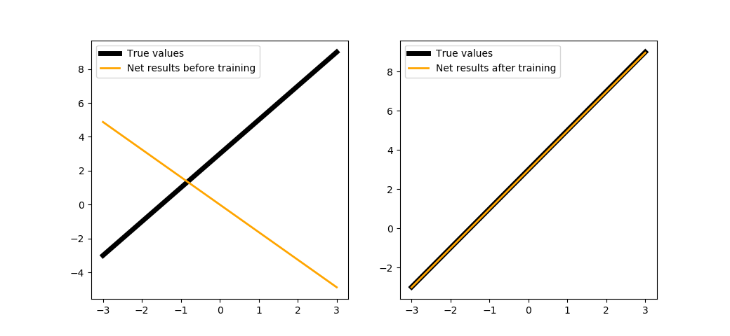
Figure 2. Comparison of network results before and after the training

As you might see, we only need to spend 100 steps of training to fully restore the function since we have the hidden layer.

Implementing the library tools¶

In this tutorial, we will not conduct parallel training, just create a separate function for training a network written in PuzzleLib:

def trainNetPL(size, steps=1000, batchsize=10, learnRate=1e-2):
    from PuzzleLib.Modules import Linear as LinearPL
    from PuzzleLib.Containers import Sequential
    from PuzzleLib.Optimizers import SGD
    from PuzzleLib.Cost import MSE
    from PuzzleLib.Handlers import Trainer
    from PuzzleLib.Backend.gpuarray import to_gpu

    np.random.seed(4321)

    net = Sequential()
    net.append(LinearPL(insize=1, outsize=size, name="layer_1", initscheme="gaussian"))
    net.append(LinearPL(insize=size, outsize=1, name="layer_2", initscheme="gaussian"))

    predictedBT = net(to_gpu(X)).get()

    cost = MSE()
    optimizer = SGD(learnRate)
    optimizer.setupOn(net)

    trainer = Trainer(net, cost, optimizer, batchsize=batchsize)

    for i in range(steps):
        idx = np.random.randint(0, 1000 - batchsize)
        x = X[idx:idx + batchsize]
        y = f(x).astype(np.float32)

        trainer.trainFromHost(x, y, macroBatchSize=batchsize,
                                onMacroBatchFinish=lambda train: print("PL module error: %s" % train.cost.getMeanError()))

    predictedAT = net(to_gpu(X)).get()

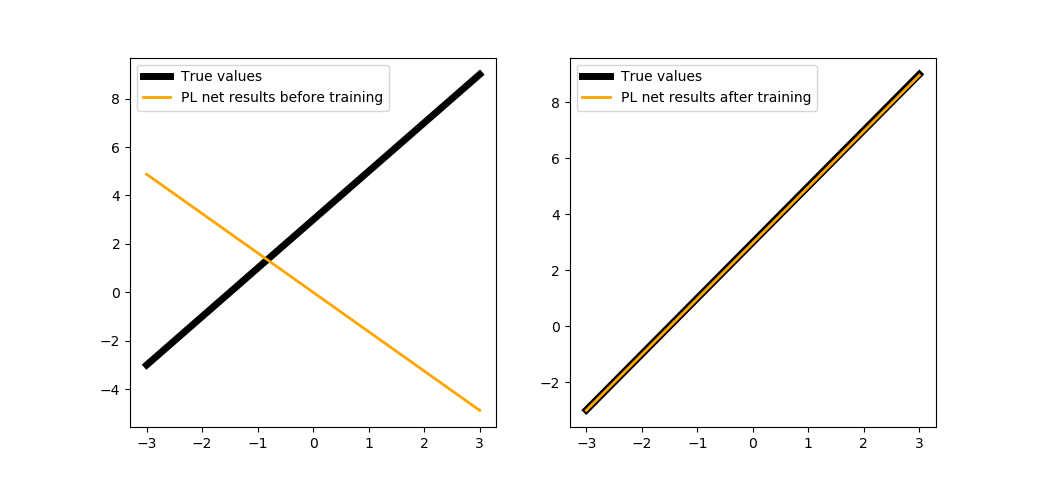
    showSubplots(
        X,
        Y,
        {
            "y": predictedBT,
            "name": "PL net results before training",
            "color": "orange"
        },
        {
            "y": predictedAT,
            "name": "PL net results after training",
            "color": "orange"
        }
    )

Figure 3. Comparison of PL network results before and after the training

Complicating the function¶

Why not complicate the function we are restoring?

def func(x):
    from math import sin
    return 2 * sin(x) + 5

f = np.vectorize(func)
Y = f(X)

trainNet(2, steps=100, batchsize=1)

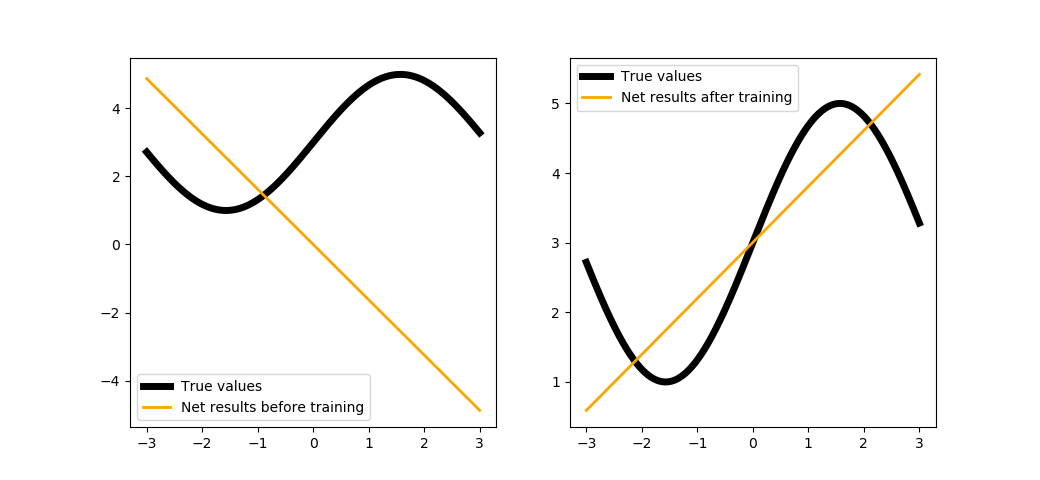
Figure 4. Comparison of network results before and after the training

You could try training with a larger number of steps, but it would not work anyway. The explanation is simple: the architecture of our network is reduced to a linear combination of linear functions (see the formulas above), i.e. it is merely a linear function. In order to solve this problem, we introduce non-linearity into the network - see the next tutorial for more information on that.