Training MNIST classifier¶

Introduction¶

In this tutorial, we will learn how to work with the PuzzleLib library by training a classifier of handwritten digits from the MNIST dataset.

Training sample¶

Go to the Yann LeCun (the creator of the MNIST dataset) website and download the following files:

t10k-images.idx3-ubyte.gz
t10k-labels.idx1-ubyte.gz
train-images.idx3-ubyte.gz
train-labels.idx1-ubyte.gz

Place and unpack the downloaded files in the directory of your choice. The extracted files contain 70,000 black-and-white images, 28 by 28 pixels each, with handwritten numbers from 0 to 9.

MNIST images example

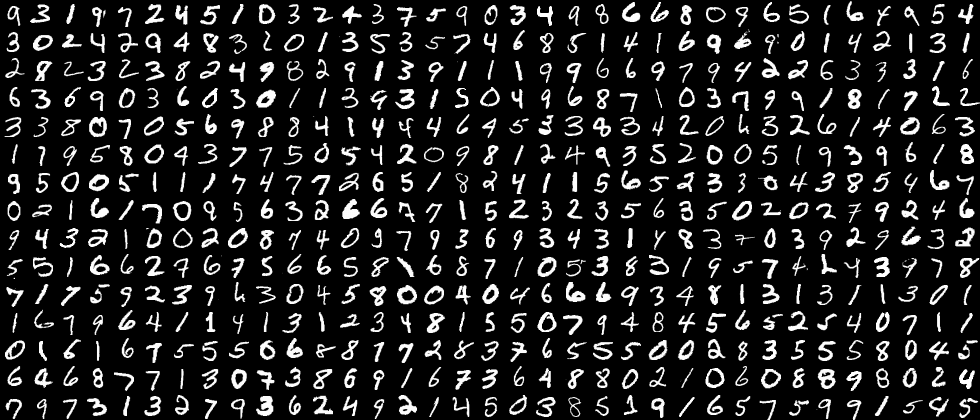
Working with MNIST is the equivalent of Hello World for working with images in machine learning. The task is to determine, what number is in the picture.

Implementation in library tools¶

Let's start with importing the system os library and numpy library - the main Python library for working with multidimensional tensors.

import os

import numpy as np

Next, we import all the classes and functions required from the PuzzleLib library.

This line imports the MNIST loader. MNIST data is stored in a specific format, and since we often use MNIST to check how the library works, the MNIST loader was added to the library, it reads MNIST files and returns them in the format required for transferring them to the neural network.

from PuzzleLib.Datasets import MnistLoader

Here we load modules required for building and training the neural network.

from PuzzleLib.Containers import Sequential
from PuzzleLib.Modules import Conv2D, MaxPool2D, Activation, Flatten, Linear
from PuzzleLib.Modules.Activation import relu
from PuzzleLib.Handlers import Trainer, Validator
from PuzzleLib.Optimizers import MomentumSGD
from PuzzleLib.Cost import CrossEntropy
from PuzzleLib.Models.Nets.LeNet import loadLeNet

The showFilters function saves neural network layers into a file. This helps to understand what features the neural network has learned.

from PuzzleLib.Visual import showFilters

path = "../TestData/"
mnist = MnistLoader()
data, labels = mnist.load(path=path)
data, labels = data[:], labels[:]
print("Loaded mnist")

Important

Please do not forget to replace the path variable with the path where you have unpacked the archive with the dataset.

Here we call the MNIST loader and it stores all the photos in data, and all their labels (i.e. indication of the specific number in the picture) in labels.

You can print to the console or check in the debugger what data and labels are. These are arrays of data in HDF format (Hierarchical Data Format), which is a convenient format for storing numerical data that we use in the library. The MNIST loader converts the original MNIST format into this format.

Since the library uses random coefficients for the neural network weights at the beginning of training, we fix the randomness before starting working with the neural network, in order to make the test script as deterministic as possible:

np.random.seed(1234)

Building the network¶

The library already implements the Lenet network and the next line shows how it can be called for further use. But for a better understanding, let's implement all the layers ourselves.

#net = loadLeNet(None, initscheme=None)

The library provides various linking modules for consolidating individual neural network computing blocks (see Containers), one of which is Sequential. This module is a container in which you can place other modules in a sequence. We named this module "lenet-5-like", which is the name of the neural network we are building. The modules do not require any obligatory names.

seq = Sequential(name="lenet-5-like")

Next, we attach the first layer to the network - the convolutional layer:

seq.append(Conv2D(inmaps=1, outmaps=16, size=3))

The append method attaches the data it receives on the input to the network.

Conv2D - convolutional layer constructor for the two-dimensional case. The layer parameters we are interested in are the following:

inmaps - number of input maps (our example images are black and white, so there is exactly one map; in case of RGB there would have been 3 maps);
outmaps - number of output maps (i.e. how many different convolutions will run through the image);
size - size of the convolutional filter (that is, the size of the window that we run through the image, collapsing it).

For more information about convolution and its parameters, please see the ConvND section.

The pooling layers usually follow the convolutional layers, MaxPool2D, in our case, which performs a two-dimensional maximizing pooling operation: just like the convolution, it runs through the image with a window, but as a result records not a linear combination of numbers from the window, but the max number that got into the window.

seq.append(MaxPool2D())

We create a pooling with the default parameters of the constructor (the window size is 2 by 2 pixels, the stride, with which we move the window on the map, is 2).

Pooling will receive 16 cards from the convolutional layer at the input, and maxpool will also give 16 cards at the output – it does not change the number of cards, but please note that maxpool reduces the size of the map, since it runs the map with a non-single stride window.

The next step is to run the nonlinear activation function set by the Activation, module on the results from the previous layer. That would be ReLU for our example:

seq.append(Activation(activation=relu))

Non-linearity is a must in a neural network, since a linear combination of numbers can yield, obviously, only a linear function from the data, and we would like the neural network not to be limited to a class of linear functions from data.

Here we join more of the same blocks (note the different Conv2D parameters).

seq.append(Conv2D(inmaps=16, outmaps=32, size=4))
seq.append(MaxPool2D())
seq.append(Activation(activation=relu))

We will get 32 cards at the output.

After that, we turn the data from the multidimensional matrix into a vector, having flattened it via the Flatten module:

seq.append(Flatten())

We perform that in order to submit the data to the input of the Linear layer (in other terminology, "fully connected layer") later:

seq.append(Linear(insize=32 * 5 * 5, outsize=1024))

The linear layer multiplies the data vector of length $l$ by the size matrix $(l, 1024)$ , outputting a vector of length 1024. As you might have guessed, the first parameter in the linear layer is the size of the input data, and the second one is the size of the output data.

The size of the input data is 32x5x5, because if multiple maxpools are used, the image size reduces to 5x5, while the number of maps has changed to 32 after the previous convolutional layer.

Then we add the activation again and another linear layer, which will receive 1024 numbers from the previous layer at the input and will output 10 numbers (the exact amount of numbers from 0 to 9):

seq.append(Activation(activation=relu))
seq.append(Linear(insize=1024, outsize=10))

Done! We have built the network.

Now the network can receive a bundle of 28x28 images for input and output a vector of 10 numbers for each. The index of the maximum of these numbers will tell you what class the network refers the image to.

Preparing for network training¶

It is time to train the neural network. We will do this using a nice variation of the gradient descent method: stochastic gradient descent with moment. The MomentumSGD module implements this training method. It will take our network and recalculate all of neural network weights in accordance with the formulas of the module.

optimizer = MomentumSGD()
optimizer.setupOn(seq, useGlobalState=True)
optimizer.learnRate = 0.1
optimizer.momRate = 0.9

We have created an optimizer, specified the network to be trained and set two internal parameters for this optimizer. All optimizers of the library have different options, for more information on that please see Optimizers. These parameters are used in the formulas for recalculating the weights of the neural network during the training.

So far, we have only created an optimizer: it does not do anything yet, as you will also need to create a trainer that would address it.

Besides the optimizer, we also need a function that would if the function erred when classifying the input photo:

cost = CrossEntropy(maxlabels=10)

We will do this with help of the CrossEntropy module that implements the cross-entropy. We consider the output of the network (10 numbers) to be a distribution of probabilities across 10 classes of digits (the probability that 0 is in the picture, ... , the probability that 9 is in the picture). We know the correct answer, so we can compare it to the network's prediction. This is exactly what cross-entropy does by producing a single number that shows how wrong the network was.

Now when we have a function that can evaluate the network error, and an optimizer that knows how to recalculate the network coefficients, knowing the error, we can create a Trainer, that will enable their interaction with each other and with the network:

trainer = Trainer(seq, cost, optimizer)

So far, we have merely created the trainer, it does not do anything yet, but we will later call its method of network training.

First let us create the Validator, which will allow us to check on the test sample how wrong the network is (we will divide the data into the training and test samples; the trainer will only see the training sample, the validator - the test one: this way we can actually assess the training quality):

validator = Validator(seq, cost)

Unlike the trainer, it does not need an optimizer, since it only has to be able to assess how wrong the seq network was on the input data. Cost will inform it on that.

Time to start with training itself.

Network training¶

We will have 15 training epochs:

for i in range(15):
        trainer.trainFromHost(data[:60000], labels[:60000], macroBatchSize=60000,
        onMacroBatchFinish=lambda train: print("Train error: %s" % train.cost.getMeanError()))

In each epoch, we first call the network training trainer.trainFromHost. The trainFromHost method performs training (i.e. updates the network coefficients). The words "fromHost" only mean that the data we provide to this method is stored in the CPU's RAM, and it must first be loaded on the GPU. There is a similar method called train, which should receive arrays that already are on the GPU.

We take 60,000 images (and their labels) and run the network training on them. The macroBatchSize parameter specifies how many photos from the entire sample we will upload to the GPU at a time. The more - the better, as it will speed the training, but sometimes the photos are large or there is not enough GPU memory, and you have to select this parameter so that the script does not crash due to the lack of GPU VRAM. The input data will be divided into macro-batches, and training will be performed upon them until the neural network has passed them all.

In the onMacroBatchFinish parameter, we specify which function should be performed when a macro-batch passes through the network. In this case, we simply print the average network error for macro-batch to the console (add the errors on each of the photos and divide by their number).

After we run all micro-batches, we print the quality of the network performance with a validator:

        Accuracy = 1.0 - validator.validateFromHost(data[60000:], labels[60000:], macroBatchSize=10000)
        print("Accuracy:", Accuracy)

Mind the following: we only give the validator the data that the network has never seen (the last 10,000 photos).

Then we reduce the network training speed by 10% (this is an empirical rule, you do not have to do this, but that would result in worse training):

optimizer.learnRate *= 0.9

Then we reduce the network training speed by 10% (this is an empirical rule, you do not have to do this, but that would result in worse training):

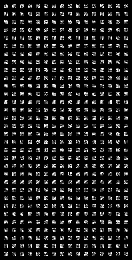
showFilters(seq[0].W.get(), os.path.join(path, "conv1.png"))
showFilters(seq[3].W.get(), os.path.join(path, "conv2.png"))

Here we took the zero and third layers of the network, applied to their weight matrices, transferred them to the CPU via the get method (since these matrices are always stored on the GPU - they are used and trained there), and then output them to the image files via the showFilters function.

After 15 epochs of training, these images are obtained:

Filters of the first convolutional layer of the lenet network (all 16 pieces)

Filters of the second convolutional layer of the lenet network (all 16x32 pieces)

The accuracy with which the network has learned classifying images:

print("Accuracy:", Accuracy)

Accuracy: 0.9924