Restoring a linear function with a single neuron

Run in Google Colab

Take a look on GitHub

Download notebook

Artificial neuron

In the previous article we talked about a model that has a $\theta$, set of parameters, which we need to optimize in order to minimize the $J(\theta)$ loss function. When it comes to deep learning, such models are actually artificial neural networks, consisting of nodes - neurons.

Usually an artificial neuron is mathematically represented as some nonlinear function from a single argument (a linear combination of all input signals) the signal of which is sent to a single output. Figure 1 shows a diagram of an artificial neuron:

Figure 1. Artificial neuron diagram

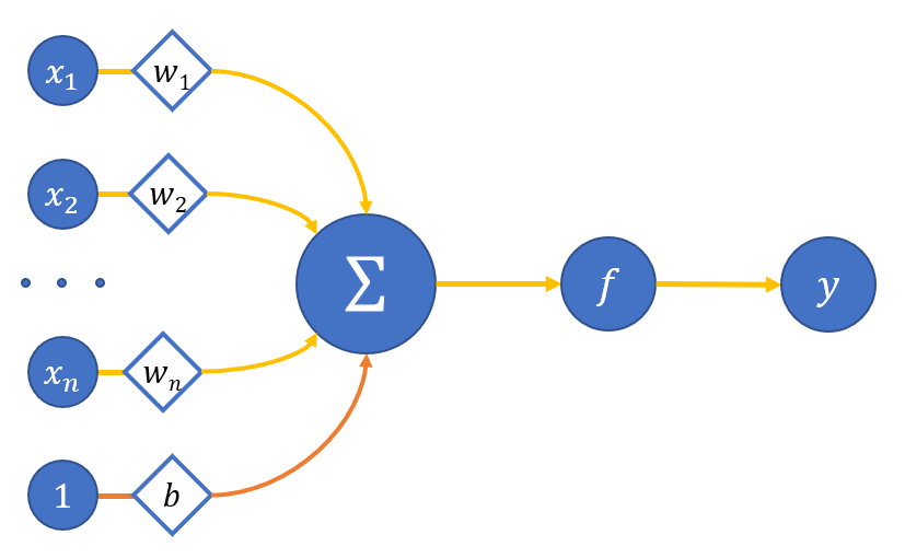
where

$x_0,...,x_n$ - neuron inputs;
$w_o,..w_n$ - weights of the corresponding inputs;
$b$ - bias weight (we equal the input of this connection to one);
$\sum$ - adder of weighted inputs;
$f$ - neuron activation function;
$y$ - neuron output.

As a result, the output of the neuron looks like this:

$$y = f(\sum_{i=1}^{n} x_iw_i + b)$$

or, if you set the bias weight as $w_0$ and the input value is $x_0$:

$$y = f(\sum_{i=0}^{n} x_iw_i)$$

A different activation function could provide an output of 1, if the linear combination of all neurons exceeds a certain value, or 0 if vice versa.
If we take such neuron for the model previously discussed, then its weights will be the exact parameters $\theta$ of the model.

We will take a model of a simplified neuron with one input and no activation function (yet) for convenience - figure 2:

Figure 2. A simplified neuron diagram

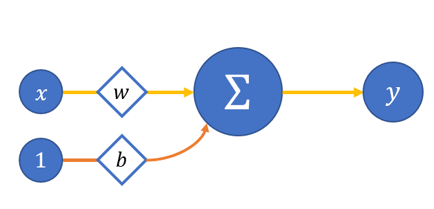
Then:

$$y = xw + b$$

which reminds the equation of a straight line a lot, so let us restore it.

To do this we have to solve the optimization problem:

$$\sum_{i=0}^{l} J(\theta) \to \min\limits_{\theta}$$

We take the mean squared as a loss function (two is added in the denominator for convenience of the further differentiation):

$$J(\theta) = \frac{1}{2N}\sum_{i=1}^N(y_i-y_i^p)^2 = \frac{1}{2N}\sum_{i=1}^N(y_i-(x_iw + b))^2$$

where

$N$ - the number of objects in the dataset;
$y_i$ - the real value for the $i$-th object;
$y_i^p$ - the value predicted by the model for the $i$-th object.

A little reminder on how we optimize the parameters:

$$\theta_{t+1} = \theta_t - \eta \cdot \frac{1}{l}\sum_{i=0}^{l} \nabla_{\theta}{J_i(\theta_t)}$$

or in case of a simplified neuron:

$$\begin{equation} w_{t+1} = w_t - \eta \cdot \frac{1}{l}\sum_{i=0}^{l} \nabla_{w}{J_i(w_t, b_t)} \end{equation}$$

$$\begin{equation} b_{t+1} = b_t - \eta \cdot \frac{1}{l}\sum_{i=0}^{l} \nabla_{b}{J_i(w_t, b_t)} \end{equation}$$

How do we find $\nabla_{w}{J_i(w_t, b_t)}$ and $\nabla_{w}{J_i(w_t, b_t)}$? All you need is to take the partial derivatives of the loss function from these parameters, which will also be the derivatives of a complex function:

$$\begin{equation} \frac{\partial{J}}{\partial{w}} = \frac{\partial{J}}{\partial{y}}\frac{\partial{y}}{\partial{w}} \end{equation}$$

$$\begin{equation} \frac{\partial{J}}{\partial{b}} = \frac{\partial{J}}{\partial{y}}\frac{\partial{y}}{\partial{b}} \end{equation}$$

We have the following analytical expressions for the selected loss function:

$$\begin{equation} \frac{\partial{J}}{\partial{y}} = -(y-y^p) \end{equation}$$

$$\begin{equation} \frac{\partial{y}}{\partial{w}} = x \end{equation}$$

$$\begin{equation} \frac{\partial{y}}{\partial{b}} = 1 \end{equation}$$

Then update the artificial neuron parameters:

$$\begin{equation} w_{t+1} = w_t - \eta \cdot \frac{1}{l}\sum_{i=0}^{l} (-(y_i-y_i^p) \cdot x_i) \end{equation}$$

$$\begin{equation} b_{t+1} = b_t - \eta \cdot \frac{1}{l}\sum_{i=0}^{l} (-(y_i-y_i^p)) \end{equation}$$

Time to implement all this in code.

A simplified neuron in code

First, we import all that we need - this is numpy for working with tensors,matplotlib.pyplot for plotting graphs and write the functions show andshowSubplots for displaying graphs on the screen:

import numpy as np
import matplotlib.pyplot as plt


def show(x, y, pred=None, title=None):
        plt.plot(x, y, linewidth=5, color="black", antialiased=True, label="True values")

        if pred is not None:
                plt.plot(x, pred, linewidth=2, color="orange", antialiased=True, label="Predicted values")
        if title is not None:
                plt.title(f'{title}')
        plt.legend()
        plt.show()


def showSubplots(x, y, *args, title=None):
        fig = plt.figure(1, figsize=[10.4, 4.8])

        for i, arg in enumerate(args):
                i += 1
                ax = fig.add_subplot(int("12{}".format(i)))

                ax.plot(x, y, linewidth=5, color="black", antialiased=True, label="True values")

                yp = arg["y"]
                name = arg["name"]
                color = arg["color"]

                ax.plot(x, yp, linewidth=2, color=color, antialiased=True, label="{}".format(name))

                ax.legend()
        if title is not None:
                fig.suptitle(f'{title}')
        fig.show()

Next, we need to set a variety of arguments for our linear function and the function itself, and for the time being:

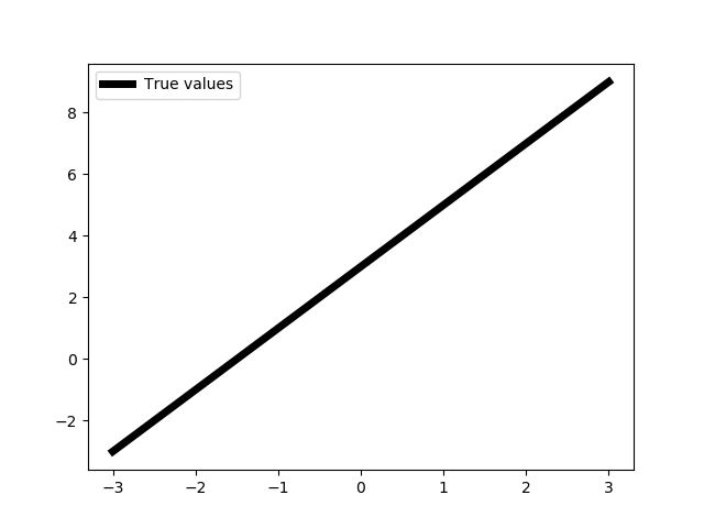
x = np.linspace(-3, 3, 1000, dtype=np.float32).reshape(-1, 1)

def func(x):
    return 2 * x + 3

f = np.vectorize(func)
Y = f(X)

show(X, Y)

Figure 3. The linear function

We do not really need np.float32 data type for now, but we will need it later.

Now we will create a simple implementation of the selected loss function - the mean squared error:

class Error:
    @staticmethod
    def value(true, pred):
        return 0.5 * np.mean((true - pred) ** 2)


    @staticmethod
    def grad(true, pred):
        c = 1 / np.prod(true.shape)
        return -(true - pred) * c

c - a coefficient of the average inverse to the number of objects in the dataset.

Finally, the artificial neuron class:

class Neuron:
    def __init__(self):
        self.w = 1
        self.b = 0

        self.inData = None
        self.data = None

        self.grad = None


    def __call__(self, data):
        return self.forward(data)


    def forward(self, data):
        self.inData = data
        self.data = data * self.w + self.b

        return self.data


    def backward(self, grad):
        self.grad = grad


    def update(self, lr=0.1):
        self.w -= self.inData * self.grad * lr
        self.b -= self.grad * lr


    def optimize(self, data, target, lr):
        prediction = self(data)

        print("Neuron error {}".format(Error.value(target, prediction)))

        grad = Error.grad(target, prediction)

        self.backward(grad)
        self.update(lr)

A bit of information on the methods implemented:

• forward - a forward propagation of data through the neuron; we need to store the input data in the class attributes here, because it will be needed during the parameters optimization (see $x$ in the weight update formula above);
• backward - something that we will need in the future, for now we just save the gradient that comes from the loss function in the class attributes;
• update - updating the neuron parameters using the aforementioned formula;
• optimize - a method that combines all the necessary operations to optimize the parameters of a neuron; lr - learning rate.

Now we can move on to the neuron training.

The neuron training

We need to initialize the neuron and compare the values it outputs with the desired function:

def trainNeuron(steps=200, learnRate=1e-2):
        neuron = Neuron()

        predictedBT = [neuron(x) for x in X]

        for i in range(steps):
                idx = np.random.randint(0, 1000)
                x = X[idx]
                y = f(x).astype(np.float32)

                neuron.optimize(x, y, learnRate)

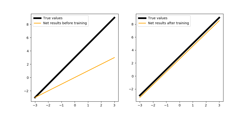
        predictedAT = [neuron(x) for x in X]

        showSubplots(
                X,
                Y,
                {
                        "y": predictedBT,
                        "name": "Net results before training",
                        "color": "orange"
                },
                {
                        "y": predictedAT,
                        "name": "Net results after training",
                        "color": "orange"
                }
        )

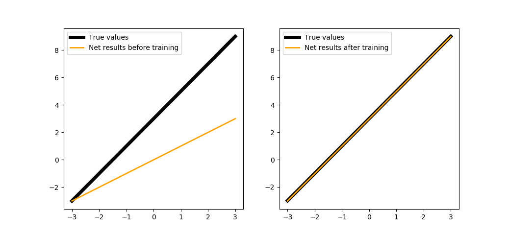
When training in 200 steps:

trainNeuron(200)

Figure 4. Comparison of neuron results before and after training in 200 steps

We could train the neuron a bit longer:

trainNeuron(500)

Figure 5. Comparison of neuron results before and after training in 500 steps

The next section will show how this was implemented in PuzzleLib.

Implementing the library tools

Now we will create a separate function to parallel the training of our neuron with the training of neuron built by the library's tools.

We will need a linear layer module through which we will simulate a neuron, an optimizer, a loss function, and a function for placing tensors on the selected device (usually that would be GPU) to_gpu to work with training a neuron on PuzzleLib:

def trainBoth(steps=1000, learnRate=1e-2):
    from PuzzleLib.Modules import Linear
    from PuzzleLib.Optimizers import SGD
    from PuzzleLib.Cost import MSE
    from PuzzleLib.Backend.gpuarray import to_gpu

Next, we declare the function that will optimize our pseudo-neuron:

    def optimizeModule(module, cost, optimizer, data, target):
        module.trainMode()

        data = to_gpu(data.reshape(-1, 1))
        target = to_gpu(target.reshape(-1, 1))

        error, grad = cost(module(data), target)
        print("PL module error {}".format(error))

        module.zeroGradParams()
        module.backward(grad, updGrad=False)
        optimizer.update()

A data reshape is necessary because PuzzleLib imposes certain requirements on the dimensions of the input data.

Let us create a pseudo-neuron and fill in the values of weights and biases so that they coincide with the neuron we created:

    neuronPL = Linear(insize=1, outsize=1)
    neuronPL.W.fill(1)
    neuronPL.b.fill(0)

Next, we initialize the loss function and the optimizer, setting the latter to a pseudo-neuron:

    cost = MSE()
    optimizer = SGD(learnRate)
    optimizer.setupOn(neuronPL)

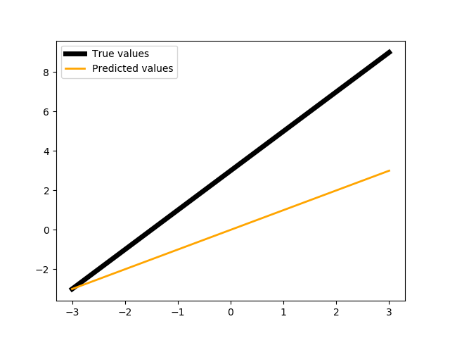
We show the values of the pseudo-neuron:

    show(X, Y, neuronPL(to_gpu(X)).get())

Finally, we will train both neurons:

    optimizer.learnRate = learnRate
    for i in range(steps):
        idx = np.random.randint(0, 1000)
        x = X[idx]
        y = f(x).astype(np.float32)

        perceptron.optimize(x, y, learnRate)

        cost.resetAccumulator()
        optimizeModule(neuronPL, cost, optimizer, x, y)

    neuronPL.evalMode()

    showSubplots(
            X,
            Y,
            {
                "y": [perceptron(x) for x in X],
                "name": "Neuron",
                "color": "orange"
            },
            {
                "y": neuronPL(to_gpu(X)).get(),
                "name": "PuzzleLib neuron",
                "color": "magenta"
            }
    )

trainBoth(500)

Figure 6. A comparison of the values of the unknown function and untrained pseudo-neuron

Figure 7. A comparison of the values of the trained neurons

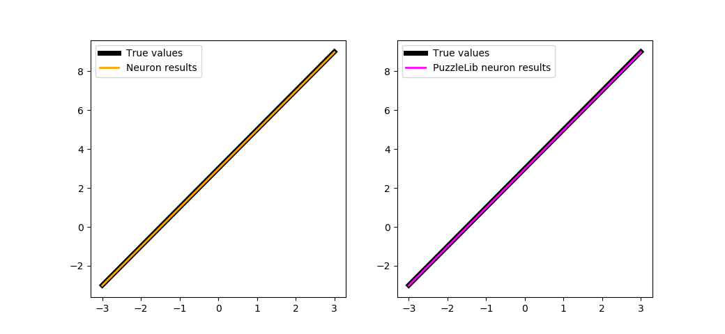
Please pay attention that the library provides handlers, which means that we do not have to create manually functions like optimizeModule, besides, they provide training on batches. If you rewrite the trainBoth function using a handler, you will get:

def trainBoth(steps=1000, learnRate=1e-2):
    from PuzzleLib.Modules import Linear
    from PuzzleLib.Optimizers import SGD
    from PuzzleLib.Cost import MSE
    from PuzzleLib.Handlers import Trainer
    from PuzzleLib.Backend.gpuarray import to_gpu

    neuronPL = Linear(insize=1, outsize=1)
    neuronPL.W.fill(1)
    neuronPL.b.fill(0)

    cost = MSE()
    optimizer = SGD(learnRate)
    optimizer.setupOn(neuronPL)

    trainer = Trainer(neuronPL, cost, optimizer, batchsize=1)

    perceptron = Neuron()

    show(X, Y, neuronPL(to_gpu(X)).get())

    for i in range(steps):
        idx = np.random.randint(0, 1000)
        x = X[idx]
        y = f(x).astype(np.float32)

        perceptron.optimize(x, y, learnRate)

        trainer.trainFromHost(x.reshape(-1, 1), y.reshape(-1, 1), macroBatchSize=1,
                                onMacroBatchFinish=lambda train: print("PL module error: %s" % train.cost.getMeanError()))

    neuronPL.evalMode()

    showSubplots(
        X,
        Y,
        {
            "y": [perceptron(x) for x in X],
            "name": "Neuron",
            "color": "orange"
        },
        {
            "y": neuronPL(to_gpu(X)).get(),
            "name": "PuzzleLib neuron",
            "color": "magenta"
        }
    )

Extra: The bias role in the neuron

What would happen if we remove the bias parameter from the neuron? We will rewrite the neuron's methods so that there is no bias during the forward propagation:

    def forward(self, data):
        self.inData = data
        self.data = data * self.w

        return self.data

trainNeuron(500)

Figure 8. Comparison of neuron results without bias before and after training

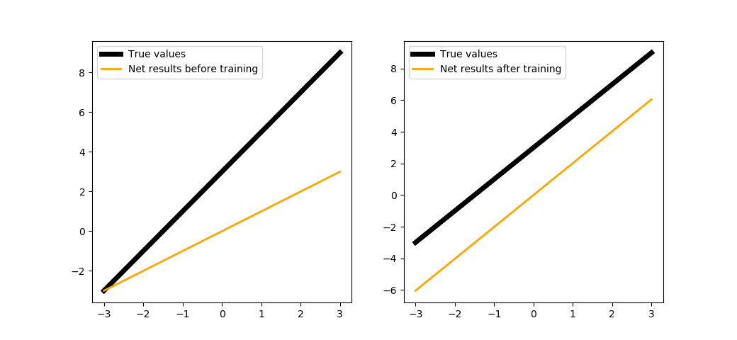
As you can see in the Fig. 8, the results provided by the neuron with no bias are in parallel with the desired function, but it lacked bias to fully restore it.